Relationship Description

This article explains the description of relationships based on the "coffee shop business scenario." The following two tables are the datasets involved.

Dataset 1: Coffee Bean Inventory Table (coffee_beans)

bean_id	bean_name	stock_kg
1	Colombia	50
2	Ethiopia	30
3	Brazil	20

Dataset 2: Coffee Sales Table (sales)

sale_id	bean_id	sale_kg
101	1	10
102	2	5
103	4	8

Association Types

Association types refer to the types of joins used when associating datasets, including left join (LEFT JOIN), inner join (INNER JOIN), right join (RIGHT JOIN), and full join (FULL JOIN).

Left Join (LEFT JOIN)

Retains all records from the left dataset, displaying NULL for unmatched records from the right side. The result of the left join between the two datasets above is: all coffee bean inventory + matching sales records (if inventory is unsold, it shows NULL). Left join result:

bean_id	bean_name	stock_kg	sale_id	bean_id	sale_kg
1	Colombia	50	101	1	10
2	Ethiopia	30	102	2	5
3	Brazil	20	NULL	NULL	NULL

Inner Join (INNER JOIN)

Retains records that exist in both datasets. The result of the inner join between the two datasets above is: only coffee beans that are both in stock and have been sold are retained. Inner join result:

bean_id	bean_name	stock_kg	sale_id	bean_id	sale_kg
1	Colombia	50	101	1	10
2	Ethiopia	30	102	2	5

RIGHT JOIN

Retains all records from the right dataset, displaying NULL for unmatched records from the left. The result of the right join between the two datasets above is: all sales records + matching inventory (if a sale was not stocked, it shows NULL).

Right join result:

bean_id	bean_name	stock_kg	sale_id	bean_id	sale_kg
1	Colombia	50	101	1	10
2	Ethiopia	30	102	2	5
NULL	NULL	NULL	103	4	8

Full Join (FULL JOIN)

Retains all results from both datasets, with unmatched parts filled with NULL. The full join result of the two datasets above is: all inventory and sales records (unmatched parts are filled with NULL). Full join result:

bean_id	bean_name	stock_kg	sale_id	bean_id	sale_kg
1	Colombia	50	101	1	10
2	Ethiopia	30	102	2	5
3	Brazil	20	NULL	NULL	NULL
NULL	NULL	NULL	103	4	8

Join Conditions

Join conditions are expressions used in join operations to specify the relationships between datasets. Typically, join conditions are based on columns within the datasets, and by comparing the values in these columns, it is determined which rows should be joined together. For example, in the aforementioned "Coffee Shop Business Scenario," there are two datasets: the "Coffee Bean Inventory Table" contains a bean_id column, and the "Coffee Sales Table" also contains a bean_id column. By using this common bean_id column, a relationship can be established between the two datasets. Correctly understanding and using join conditions is key to efficient model queries.

Single-Column Association

The association condition between two datasets can be described as the equality of a single column. In the example of the "Coffee Shop Business Scenario," the association condition can be written as: {{Coffee Bean Inventory}}.{bean_id} = {{Coffee Sales}}.{bean_id}. In the HENGSHI SENSE data model interface, users can configure this association condition by selecting columns on the Simple Condition page, or by writing expressions on the Expression Condition page.

Multi-Column Join

The join condition between two datasets may require equality on multiple columns. For example, consider the following two datasets: Coffee Orders Table and Coffee Inventory Table. When we want to query the inventory status of the coffee involved in each order, we need to join based on both the coffee type (coffee_type) and roast level (roast_level) columns. The join condition should be written as: {{coffee_orders}}.{coffee_type} = {{coffee_inventory}}.{coffee_type} AND {{coffee_orders}}.{roast_level} = {{coffee_inventory}}.{roast_level}. In the HENGSHI SENSE data model interface, users can configure this join condition by selecting columns on the Simple Condition page, or by writing an expression on the Expression Condition page.

Dataset 3: Coffee Orders Table (coffee_orders)

coffee_type	roast_level	quantity
Colombia	Medium Roast	5
Ethiopia	Light Roast	3
Brazil	Dark Roast	7

Dataset 4: Coffee Inventory Table (coffee_inventory)

coffee_type	roast_level	available_quantity
Colombia	Medium Roast	32.5
Ethiopia	Light Roast	18.2
Brazil	Dark Roast	12.8
Guatemala	Medium Roast	9.5

According to the above join condition, select the left join type: the Coffee Orders Table is left joined with the Coffee Inventory Table, and the resulting data is as follows:

coffee_type	roast_level	quantity	available_quantity
Colombia	Medium Roast	5	32.5
Ethiopia	Light Roast	3	18.2
Brazil	Dark Roast	7	12.8

Non-Equi Join

In addition to using "equals" for equi joins, you can also use other comparison operators or nested functions to perform non-equi joins. For example, to find coffee products that fall within the price range acceptable to customers, a non-equi join is required. The join condition is: {{coffee_products}}.{price} >= {{customer_preferences}}.{min_price} AND {{coffee_products}}.{price} <= {{customer_preferences}}.{max_price}. In the HENGSHI SENSE data model interface, users can only configure this join condition by writing an expression on the Expression Condition page.

Dataset 5: Coffee Products Table (coffee_products)

product_id	product_name	price
CP001	Colombia Special	58
CP002	Ethiopia Gesha	85
CP003	Brazil Yellow Bourbon	42

Dataset 6: Customer Preferences Table (customer_preferences)

customer_id	min_price	max_price
CU1001	30	80
CU1002	50	120
CU1003	20	60

According to the above join condition, select the inner join type. When the Coffee Products Table is inner joined with the Customer Preferences Table, the resulting data is as follows:

product_id	product_name	price	customer_id	min_price	max_price
CP001	Colombia Special	58	CU1001	30	80
CP001	Colombia Special	58	CU1002	50	120
CP001	Colombia Special	58	CU1003	20	60
CP002	Ethiopia Gesha	85	CU1002	50	120
CP003	Brazil Yellow Bourbon	42	CU1001	30	80
CP003	Brazil Yellow Bourbon	42	CU1003	20	60

Association Cardinality

The association cardinality of a relationship reflects the data characteristics of the related columns on the "from" and "to" sides. The "one" side indicates that each row in the column contains a unique value, while the "many" side means that multiple rows in the column can contain duplicate values. The association condition is the key basis for determining cardinality. There are four types of association cardinality: one-to-one, one-to-many, many-to-one, and many-to-many. If the relationship from Dataset A to Dataset B is one-to-many, it means that introducing Dataset B will cause data expansion in Dataset A.

Determining the Cardinality of Relationships

Cardinality Determination under Simple Join Conditions

When the join condition is a simple condition, we can define the relationship cardinality by checking whether the values in the relevant columns are unique. The following example uses the Department Member table and the User Information datasets for illustration. The join condition between these two datasets is {{Department Member}}.{user_id} = {{User Information}}.{id}. In the Department Member dataset, there are multiple rows containing the same "user_id", which indicates that the Department Member dataset should be defined as the "many" side of the relationship. In the User Information dataset, each row's "id" is unique, so the User Information table should be defined as the "one" side. The cardinality between Department Member and User Information is determined to be "many-to-one".

Dataset 7: Department Member (depart_member)

l1	l2	user_id
Sales	Sales Dept 1	1
Sales	Sales Dept 2	2
Sales	Sales Dept 3	3
Sales	Marketing	1
Sales	Key Account	2
Marketing	Marketing	1

Dataset 8: User Information (user)

id	name
1	jack
2	tom
3	amy

Cardinality Determination Under Complex Join Conditions

When the join condition is complex, we can assist in determining cardinality by adding a virtual column. Take the Sales Orders table and the Month Info datasets as an example. The join condition between these two datasets is trunc_month({{Sales Orders}}.{day}) = {{Month Info}}.{month}, where the trunc_month function is used to get the first day of the month for a given variable. We add a virtual column trunc_month({{Sales Orders}}.{day}) to the Sales Orders table. If multiple rows have the same value in this column, it means the "Sales Orders" table should be defined as the "many" side of the cardinality. In contrast, each row in the "Month Info" table has a unique "month" value, so the "Month Info" table should be defined as the "one" side. Therefore, the cardinality between Sales Orders and Month Info is determined as many-to-one.

Dataset 9: Sales Orders (orders)

day	order_num	trunc_month({{Sales Orders}}.{day})
2023-01-01	200	2023-01-01
2023-01-02	150	2023-01-01
2023-01-04	300	2023-01-01
2023-02-01	100	2023-02-01
2023-02-05	80	2023-02-01
2023-02-06	90	2023-02-01
2023-01-01	200	2023-01-01

Dataset 10: Month Info (date)

month
2023-01-01
2023-02-01
2023-03-01

Impact of Join Cardinality on Model Calculations

The "many" side in a join cardinality will cause data expansion on the other side, so setting different cardinality types in the model determines the execution logic of the join calculation. The core rules are as follows:

1. The model table must always participate in calculations under any circumstances. All datasets along the path from the model table to the dataset used by the measure will also participate in the calculation. Whether the nodes after the dataset used by the measure participate in the calculation is determined by the join cardinality.
2. To ensure the correctness of each measure, if introducing Measure B while calculating Measure A causes data expansion in the dataset where Measure A resides, then Measure A and Measure B should be calculated separately.

In the following explanation, assume the left table is the model table and the right table is the subordinate table. Different join cardinalities will result in different execution logics:

1. One-to-One: This cardinality type represents an equal relationship and will not cause data expansion during the data join process. All calculations based on the left and right tables are founded on the join result of the left and right tables.
2. One-to-Many: This cardinality type means that joining with the right table will cause data expansion in the left table. The calculation basis for measures related only to the left table is the left table itself, while the calculation basis for other measures is the join result of the left and right tables.
3. Many-to-One: This cardinality type means that joining with the left table will cause data expansion in the right table. However, since the model table always participates in the calculation, all calculations based on the left and right tables are founded on the join result of the left and right tables.
4. Many-to-Many: Both the left and right tables will experience data expansion due to the join, but the model table must always participate in the calculation. The calculation basis for measures related only to the left table is the left table itself, while the calculation basis for other measures is the join result of the left and right tables.

Activation Mechanism

The model contains a model table and multiple sub-tables. In scenario analysis based on this model, the model table will always be included in the calculation. However, whether the sub-tables are included in the calculation depends on the activation mechanism of the sub-tables. The activation mechanism determines how datasets collaborate with each other during the calculation process. There are two types of activation mechanisms: associate on demand and always associate.

On-Demand Association

On-demand association is the default activation mechanism for relationships. Its core feature is that the right table only participates in the calculation process when its fields are used in the analysis. This mechanism embodies the concept of "on-demand invocation," allowing the right table data to be flexibly introduced based on actual calculation needs, thereby avoiding unnecessary resource consumption.

Always Associate

The "Always Associate" mechanism can only be set when the cardinality of the relationship is "one-to-one" or "many-to-one." The rule is that as long as the left dataset is used in the calculation process, the right dataset will automatically participate in the calculation. This mechanism ensures that the data on the right always works in conjunction with the data on the left. This feature is typically used in scenarios where datasets are used to restrict data permissions.

Filter Conditions

Filter conditions after model association refer to the filtering rules set after completing the association operations between data models. When data models are associated, different structured datasets are combined based on their relationships, which may result in a large amount of data. Some of this data may not be necessary for the current specific analysis scenario. At this point, filter conditions are needed to screen the associated data.

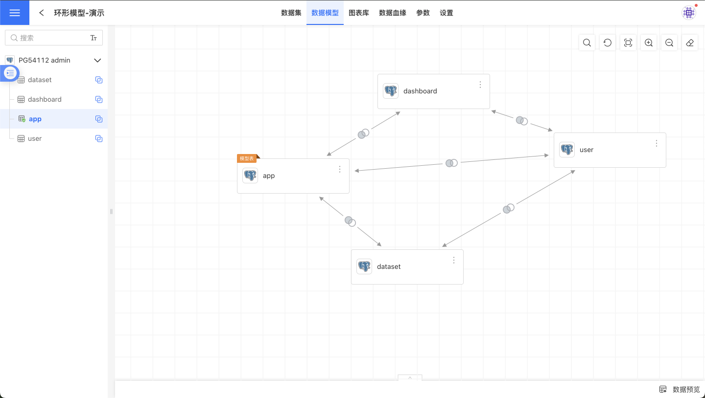
Enabling the Ring Model

There are two options for enabling the ring model feature, which determine whether the current child table can have multiple upstream datasets. Independent Association means the current child table can only have one upstream dataset, while Shared Association means the current child table can have multiple upstream datasets. Enabling Shared Association is typically used in scenarios with multi-dimensional tables and multiple fact tables.

In the scenario shown below, the user dataset serves as user information and is associated with the app, dataset, and dashboard datasets. This allows for simultaneous analysis of the app, dataset, and dashboard datasets from the user dimension.

Limitations of the ring model:

1. The association cardinality between other tables and the child table with "Shared Association" can be many-to-one (many:1) or one-to-one (1:1).
2. The relationship path starts from the model table and ends at the child table with "Shared Association"; no other child tables can follow after the child table with "Shared Association".
3. The child table with "Shared Association" does not support renaming.
4. In a single model, the same dataset can only exist as a "Shared Association" child table once.