Data Integration
Data integration provides ETL (Extract-Transform-Load) functionality, allowing data from different sources to be extracted, filtered, transformed, formatted, calculated with additional columns, associated, merged, aggregated, and then output to the user-specified data source for subsequent exploration and analysis.
Data Processing Workflow
The data processing workflow for data integration projects is roughly divided into three parts: connecting data, cleaning and transforming data, and outputting data.
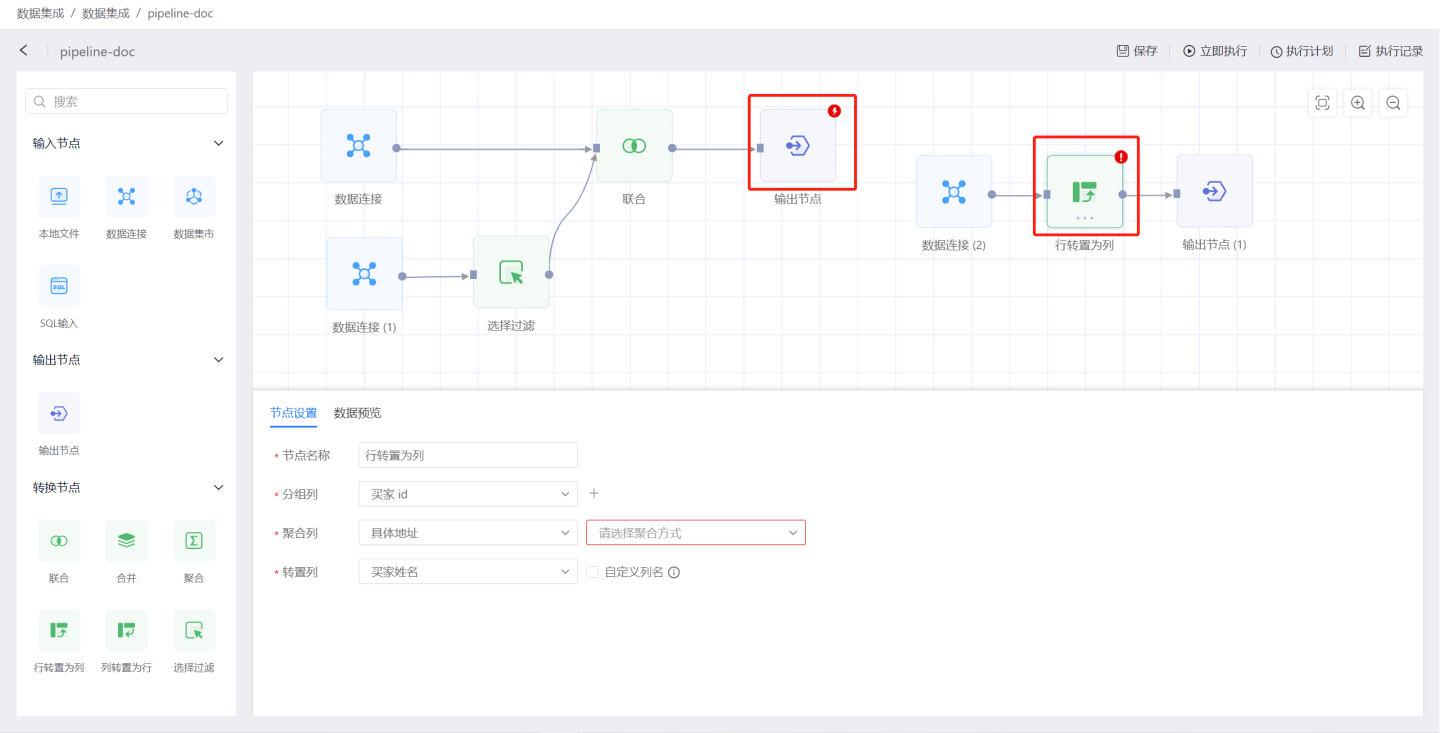
The data integration page is shown in the figure below. The red box area on the left is the node area, where all nodes can be dragged into the blue box canvas area in the middle. Nodes are connected within the canvas area to complete the data flow transmission between nodes, ultimately flowing to the output node. Clicking on a node in the canvas allows you to configure the node. The top right corner of the canvas contains the Project Execution button. 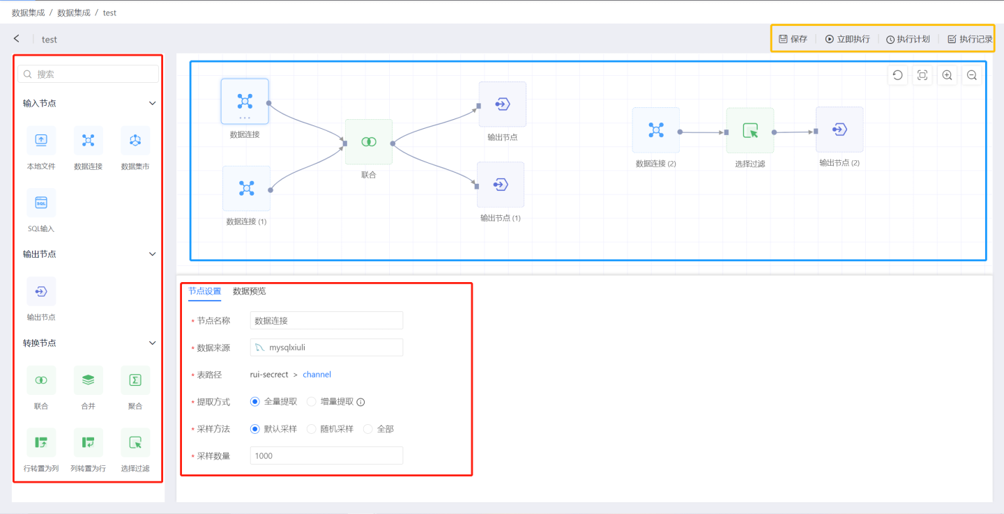
Data Integration Project Creation Process
The following describes the process of creating a data integration project. You can follow the guidance below to create a project.
Create a project.
On the data integration page, click theNew Projectbutton in the upper right corner. A new project operation box will pop up. Enter the project name in the popup window and select the lowest-level directory of the data connection as the default output path for the output node in theDefault Output Path.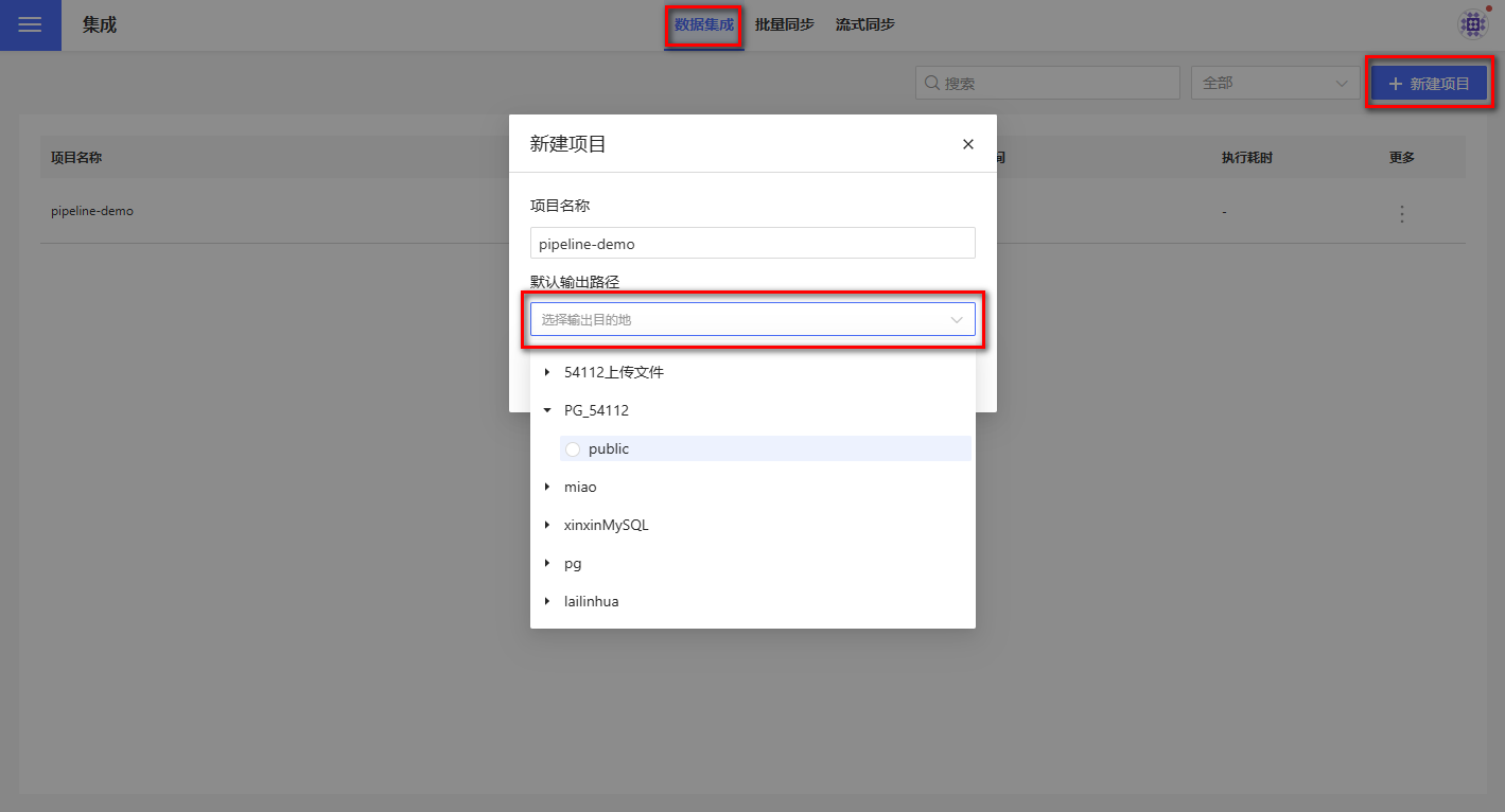
Create input nodes.
Select the input node type, drag it onto the canvas, and choose the data source. Supported input nodes include Local Files, Data Connections, Data Marketplace, and SQL Input.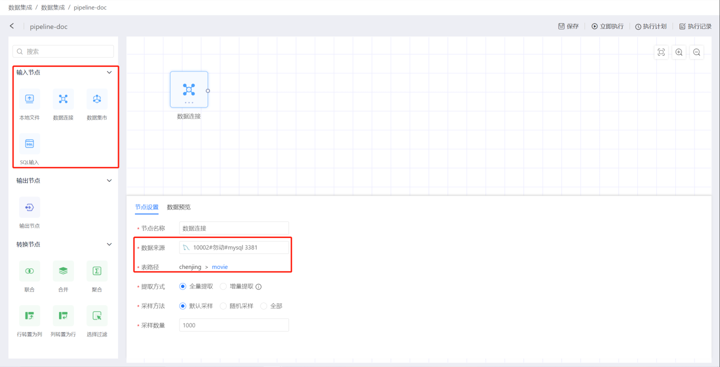
Configure the input node. Set the node name, extraction method, sampling method, and then preview whether the data meets the configuration requirements. In the example, full extraction is selected, the default sampling method is used, and 1,000 rows of data are taken. For detailed configuration instructions, please refer to Input Nodes.Add transformation nodes.
Select a transformation node, drag it onto the canvas, connect it to the upstream data source, and perform transformation operations on the data. Supported transformation operations include Union, Merge, Aggregate, Transpose Rows to Columns, Transpose Columns to Rows, and Filter Selection.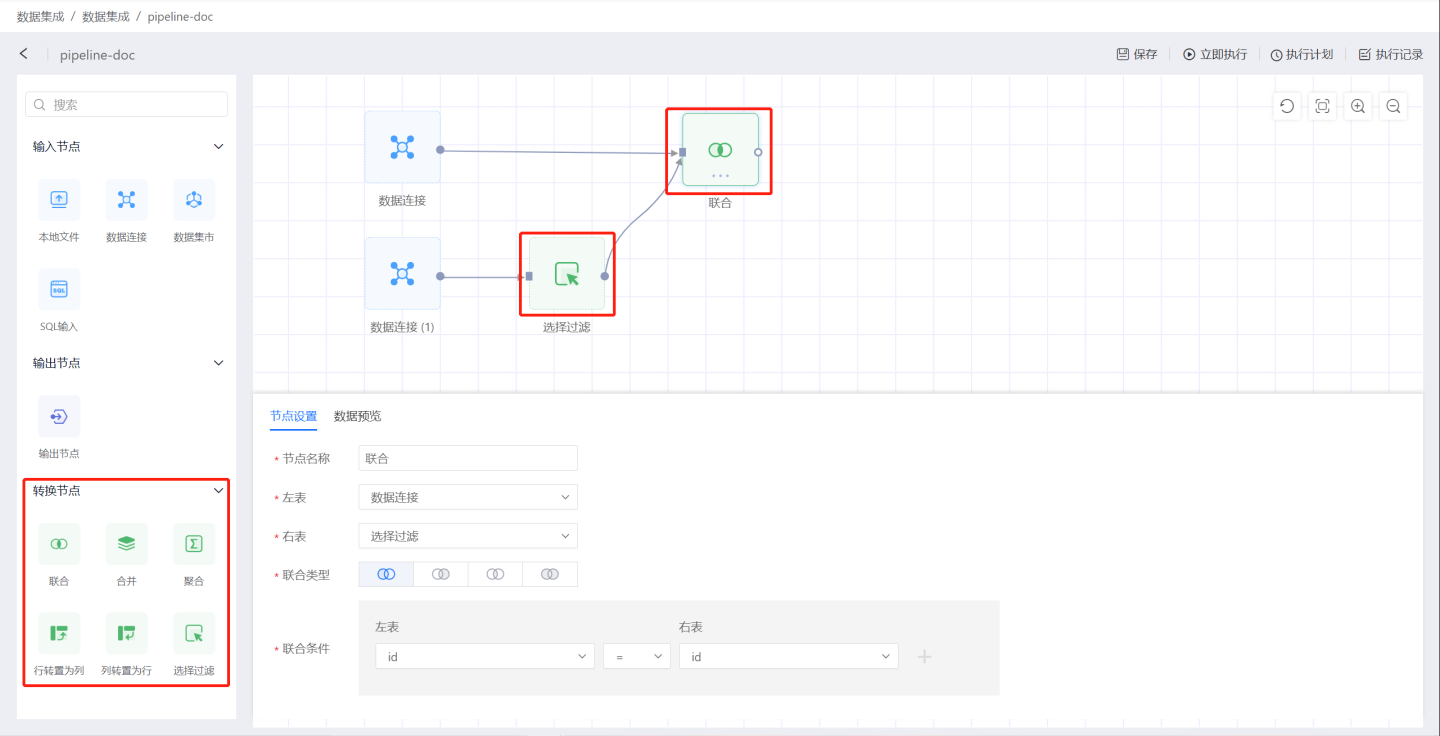
Create output nodes to store data.
Drag an output node onto the canvas, connect it to the upstream data, and set the location and table name for storing the data output.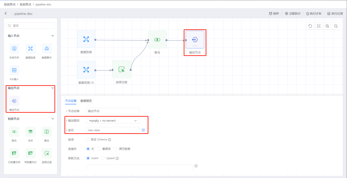
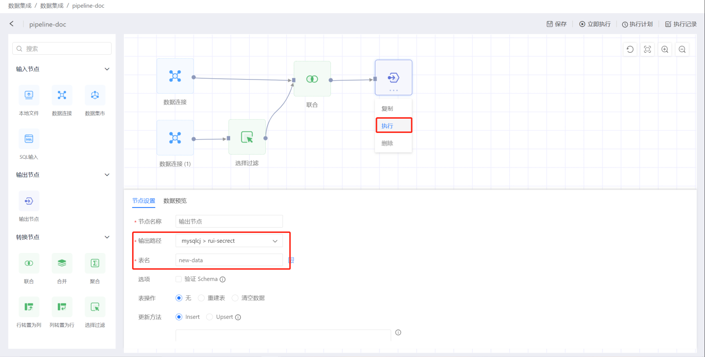
Configure the output node. Set schema validation, table operation methods, update methods, load pre-SQL, and load post-SQL. For detailed configuration instructions, please refer to Output Nodes.Complete the setup of a data processing flow following the steps above. Click the three-dot menu on the output node to execute the task. Once the task is completed, you can view the data processing results.
Build other data processing flows within the project.
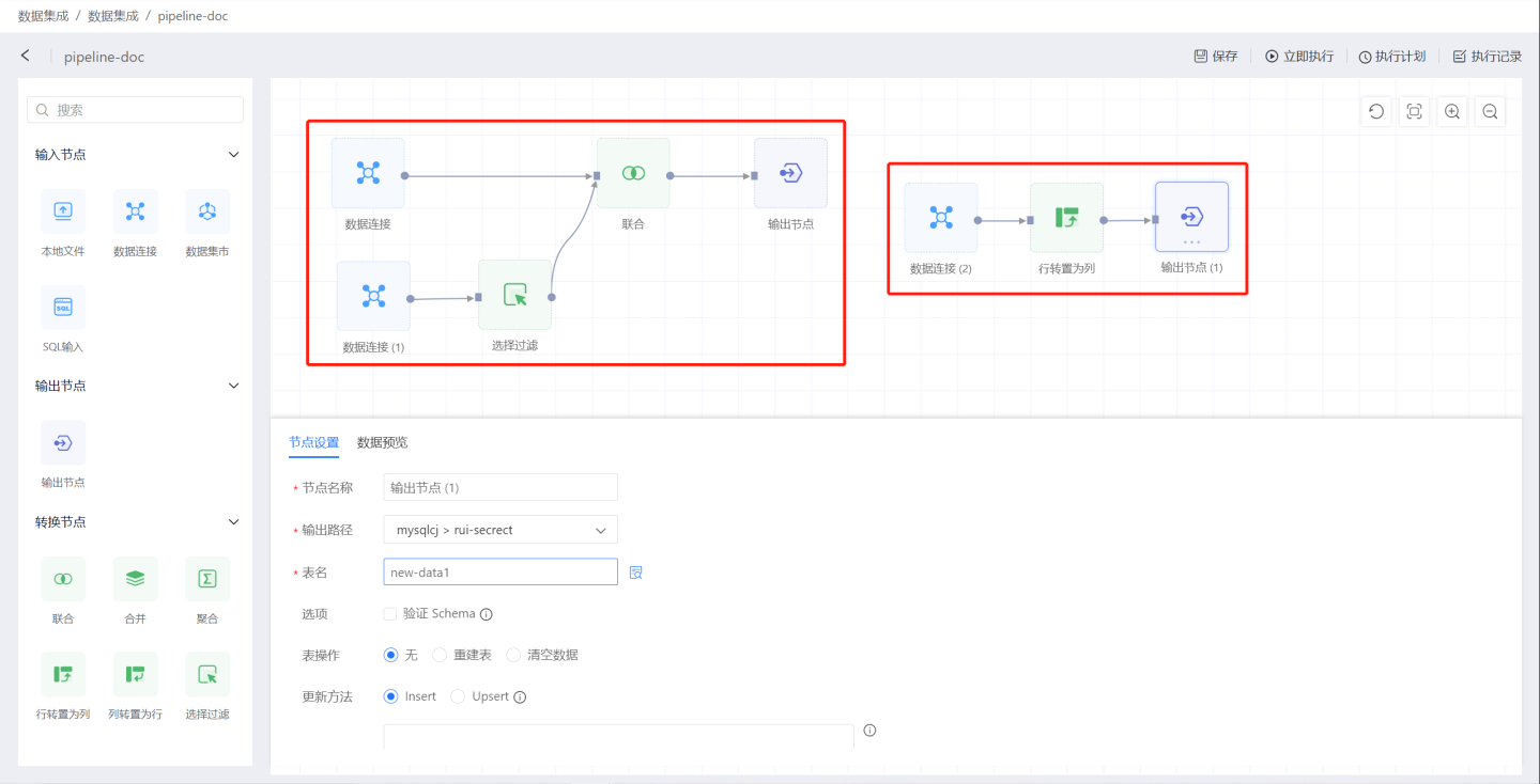
The example above briefly demonstrates the process of creating a data processing flow in data integration. Below, we will provide a detailed introduction to the functions and configurations of each node in the data processing flow.
Input Node
The data source for data integration is implemented through the input node. An input node can connect to multiple transformation nodes or output nodes. Below is a detailed introduction to the functionality and configuration of the input node.
Input Types
Input nodes support four types: local files, data connections, data marts, and SQL input.
Local File
When adding a local file as an input node, the system supports uploading files in two formats: CSV and Excel.
CSV Format Files
When uploading files in CSV format, you can configure the file's delimiter and encoding according to the local file format. Additionally, you can set the header, select rows and columns, and configure row-column inversion as needed.
Excel Format Files
When uploading files in Excel format, you can select the desired sheet from a multi-sheet file. Then, you can set the header, select rows and columns, and configure row-column inversion as needed.
Data Connection
When adding tables from a data connection as input nodes, there are two main categories: built-in data connections and user data connections:
Built-in Connections: These are the engine data connections embedded within the HENGSHI SENSE system.
User Connections: These are data connections created by the user or authorized data connections that the current account has permission to access. Users can select a table from the connection as an input node.
Tip
If the user only has view name permission for a table, the Add button will be grayed out during data preview, and the table cannot be used as an input node.
Dataset Marketplace
You can select datasets from the Dataset Marketplace as input nodes and export the results of the datasets to output sources, making it convenient for customers to explore and use.
SQL Input
The SQL Input node refers to the data content of an input node defined using SQL language. First, select the data connection, and then define the data object using SQL language.
Tip
For SQL Input nodes, users need to have read-only (RO) permissions for the entire connection associated with the connection; otherwise, execution will fail.
Data Extraction Methods
Data import is divided into two methods: Full Extraction and Incremental Extraction.
Full Extraction
Full Extraction extracts all the data from the input node each time.
Incremental Extraction
Incremental Extraction requires selecting an incremental field. During extraction, only data with incremental field values greater than the maximum value of the incremental field in the currently imported data will be extracted. The incremental field must be monotonically increasing. If multiple incremental fields are selected, they will be combined in the order they are added to form a multi-field combination, which must also be monotonically increasing. For example, a combination of year field, month field, and day field. Using unrelated fields cannot form a valid incremental field combination. The maximum value of the incremental field is recorded in the input node and is unrelated to the output node. After setting the incremental field, the first execution will still perform a full extraction because there is no maximum value record during the initial execution.
Tip
The incremental field or incremental field combination must be monotonically increasing; otherwise, it is not suitable for incremental extraction, which may result in missing data. For incremental extraction, it is recommended to use entity fields from the database table, and the database should have corresponding indexes added. Otherwise, query performance may not be better than full extraction. For SQL input nodes, the query performance of incremental extraction may not be significantly better than full extraction. During incremental extraction, Data Preview will only display data with values greater than the maximum value of the incremental field in the output table. If the input table does not contain data greater than the maximum value of the incremental field, the preview data will be empty.
Data Batch Extraction
When the amount of data being extracted is relatively large, the data import time may exceed the query timeout of the source database, resulting in data extraction failure. In this case, you can configure the option ETL_SRC_MYSQL_PAGE_SIZE (MySQL) or ENGINE_IMPORT_FROM_PG_BATCH_FETCH_SIZE (PostgreSQL) to set the maximum limit for data extraction at one time. If the limit is exceeded, the data will be extracted in batches. Currently, only MySQL and PostgreSQL data sources support batch extraction.
Tip
Please contact technical personnel to configure ETL_SRC_MYSQL_PAGE_SIZE or ENGINE_IMPORT_FROM_PG_BATCH_FETCH_SIZE.
Data Sampling
Data sampling is a debugging feature that facilitates previewing the data extracted from the input node during the current data processing, improving the efficiency of operation nodes. The sampling quantity does not affect the actual amount of data extracted during runtime. Generally, the default configuration is sufficient.
Sampling methods are divided into three types: Default Sampling, Random Sampling, and All.
Default Sampling: The query is submitted to the database for execution, and the results are extracted in the default output order of the database, selecting the specified number of samples sequentially.
Random Sampling: Randomly extracts the specified number of data entries from the sampling quantity. This requires database support for random sorting and is only needed in scenarios where the representativeness of the sampled data is a concern. It is generally not used.
All: When the sampling method is set to "All," all data from the database is extracted without manually setting the sampling quantity. This is not recommended as it may affect performance when the data volume is large. Consider using "All" sampling only when a large sampling quantity still fails to retrieve the required data.
Output Node
After data processing, the output node stores the data into the specified database. Below is a detailed introduction to the output node.
Basic Information
The output node's basic information includes the node name, output path, and table name.
Node Name: Refers to the name of the output node on the canvas, which can be modified.
Output Path: The path where the data is stored. By default, it is the destination selected when creating the project, but it can be modified. Currently supported destinations include MySQL, Apache Doris, StarRocks, SelectDB, PostgreSQL, Greenplum, Oracle, Saphana, SQL Server, Cloudera Impala, Amazon Redshift, Amazon Athena, Alibaba Hologres, Presto, ClickHouse, Dameng, TDSQL MySQL, TDSQL PostgreSQL, GBase 8a, GaussDB, OceanBase, and AnalyticDB MySQL as output node storage paths. The connection settings for the output must have the Allow Write Operations option enabled.
Table Name: The name of the table where the data is stored in the database after the output node is executed. The default table name is Output Node.
Tip
The current user must have read-write (RW) permissions for the output directory or output table for the project to execute successfully.
Output Settings
Output settings include: Validate Schema, Table Operations, Update Method, Pre-load SQL, Post-load SQL. The execution order in the output node is Pre-load SQL -> Validate Schema -> Table Operations -> Update Method -> Post-load SQL.
Validate Schema
Validating the Schema ensures that the input fields and output table fields match.
When
Validate Schemais selected, the output node will only run if the schema matches; otherwise, an error will occur during the execution of the output node. The matching rules are as follows:- The number and names of fields on both sides must be identical. If the number or names differ, it is considered a mismatch.
- For fields with the same name, the original type must be converted to the same HENGSHI type. HENGSHI types (Number/Text/Date/Boolean/JSON) are identified by the
typefield in the backend.
When
Validate Schemais not selected, the output table will be processed as follows:- For fields missing in the input table, the output table fields will be filled with null.
- For extra fields in the input table, these fields will be added to the output table and filled in new rows, while existing rows in the output table will be filled with null.
- If field names are the same but field types are incompatible (e.g., the output table field type is Number while the input table field type is String), the project execution will fail.
- If field names are the same and field types are compatible (e.g., the output table field type is Text while the input table field type is Number), the project execution will succeed.
Table Operations
Table operations are defined as actions performed on the output table when it already exists. This option does not apply when creating a new table.
None: Indicates no operations will be performed on the output table, leaving it as is.
Rebuild Table: Deletes the original output table and rebuilds the table according to the input field schema.
Clear Data: Clears all data in the table.
Tip
- During the actual operation of rebuilding a table, a temporary table is first created in the output path to store the data processing results. Once the data processing is complete, the original output table is deleted, and the temporary table is renamed to the original output table. However, in the case of the TDSQL-MySQL data source, since it does not support temporary table renaming operations, the original output table must be deleted first. If an exception occurs during the data processing, the new output table will have no data. Therefore, please exercise caution when choosing this option with the TDSQL-MySQL data source.
Update Method
Define how the input data is updated into the output table.
Insert: Insert data into the output table, i.e., append to the output table.
Upsert: Upsert = Update + Insert, update existing rows and insert new rows.
Tip
When selecting Upsert, you must set key fields to identify rows that already exist in the output table. For existing rows, update them based on the key fields. For non-existing rows, directly insert them into the output table.
Key Fields
Key fields are used as primary keys and distribution keys. Key fields serve two purposes:
- Used as primary keys during incremental updates.
- Used as primary keys and distribution keys when creating tables. If table creation attributes are configured during table creation, the configuration of the table creation attributes takes precedence, and the settings of key fields will not take effect.
Table Properties
During the process of creating a data synchronization table, you can customize partition fields and index fields to distribute data storage. Table properties only take effect during the initial table creation. Currently supported data sources for table properties include Greenplum, Apache Doris, StarRocks, and ClickHouse.
Example:
DISTRIBUTED BY (username)
PARTITION BY RANGE (username)
( START (varchar 'A1') EXCLUSIVE
   END (varchar 'A8') INCLUSIVE,
  DEFAULT PARTITION extra
);You can first click the icon next to the table properties to obtain sample syntax for the corresponding data source. Based on the sample, you can make necessary modifications according to the syntax of the specific data source. Clicking "Test Table Creation" will create a temporary table with the current properties to test the syntax correctness.
Pre-load SQL
The SQL executed before loading the extracted input data into the output table is the first configuration of the output node. It can be any SQL that complies with the syntax of the target data source, such as creating tables, clearing tables, inserting flags, deleting indexes, etc. Add as needed based on business requirements.
Post-load SQL
The SQL executed after loading the extracted input data into the output table is the final configuration of the output node. It can be any SQL that complies with the target data source syntax, such as inserting flags, rebuilding indexes, etc. Add as needed based on business requirements.
Transformation Node
The transformation node is the "T" part of ELT, enhancing data integration capabilities and helping enterprises meet the needs of agile business preprocessing. By incorporating transformation nodes into the data processing workflow, users can perform various data cleaning and transformation operations in a visual and low-threshold manner, fulfilling flexible data processing requirements.
Union
The Union node enables the union processing of two data sources. As shown in the figure, connect the data sources to be merged, then select the union type and union conditions to complete the union node operation. You can preview the data to check the processing results.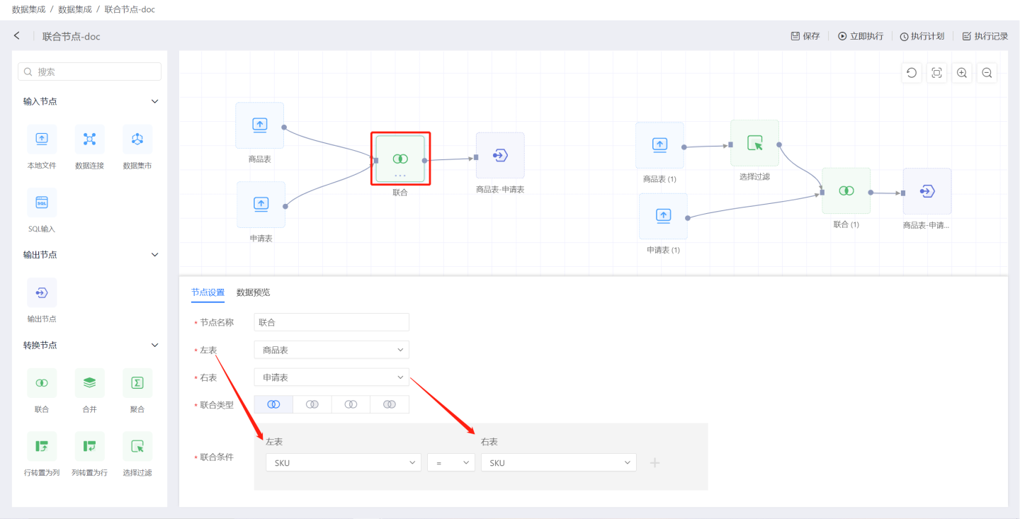
Union node configuration details:
- Node Name: Default is
Union, but users can modify it. - Left Table: The data source for the union operation, designated as the left table.
- Right Table: The data source for the union operation, designated as the right table.
- Union Type: Supports four types of connections: left join, right join, inner join, and outer join.
- Union Conditions: You can set one or more union conditions.
Tip
- The Union node only supports union operations between two data nodes.
- If the data connections of the two nodes are different, the system will first import the data from both nodes into the internal engine before performing the association operation.
Merge
The merge node combines information from multiple data nodes into a single table. As shown in the figure, the nodes of the order tables from January to March are connected to the merge node to generate a quarterly order table. 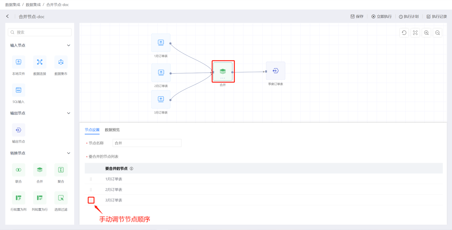
Configuration details for the merge node:
- Node Name: Defaults to
Merge, but users can modify it. - Merge Node List: The data nodes to be merged, sorted according to the connection order. Manual adjustment of the order is supported.
Merge Rules:
- The first node in the merge node list is used as the base data. The field names, field types, and field order of this node will serve as the field names, field types, and field order of the output data.
- Starting from the second node, the following rules are applied to merge it with the first node:
- If the field name matches the field name of the first node and the types are the same, the field content is filled into the corresponding field of the output data.
- If the field name matches the field name of the first node but the types differ, the system attempts to convert the type. If the conversion succeeds, the field content is filled into the corresponding field of the output data. If the conversion fails, the corresponding field in the output data is filled with NULL.
- If the field name does not match the field name of the first node, the field is discarded.
- If a field from the first node does not exist, the corresponding field in the output data is filled with NULL.
- Manual adjustment of the merge node order is supported.
Tip
- If the upstream nodes originate from different data connections, the system will first import all upstream node data into the internal engine before performing the merge operation.
Aggregation
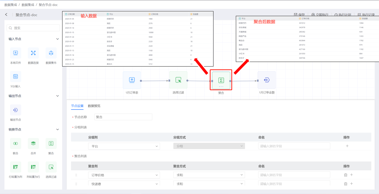
The aggregation node performs aggregation operations on the input data source. As shown in the figure, the order price and delivery fee in the January order table are aggregated to generate the order amount table.
 Explanation of aggregation node configuration:
Node Name: Default is
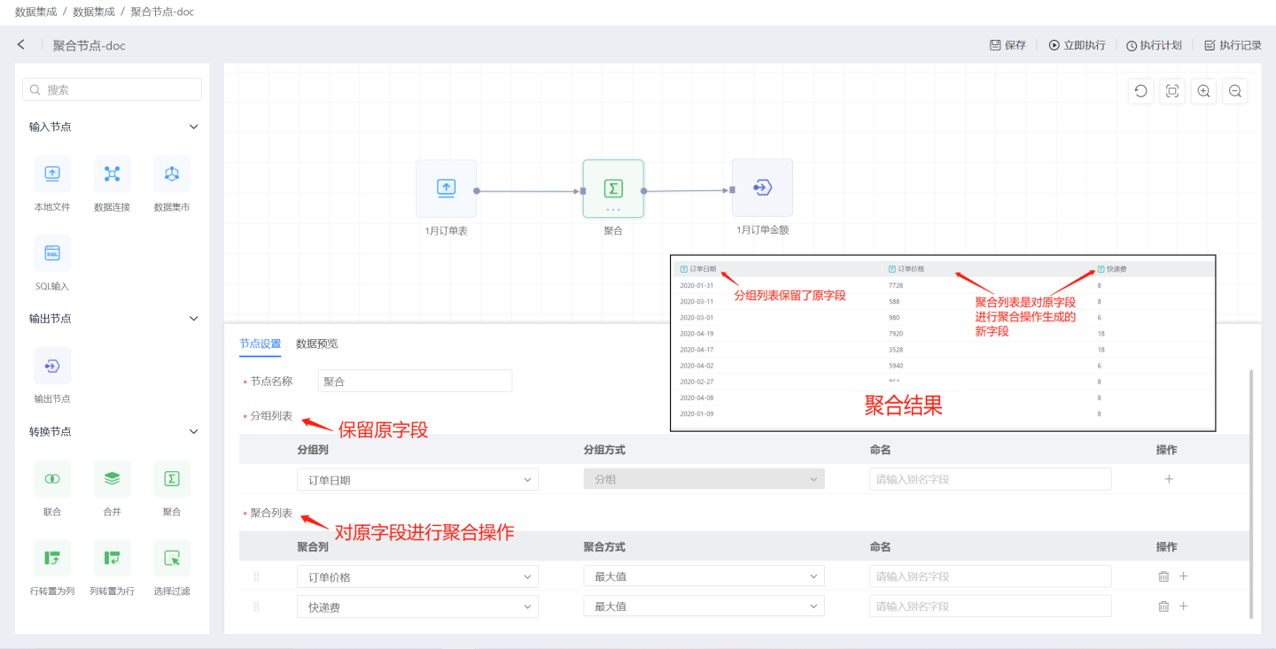
Aggregation, and users can modify it.Group List: Retain fields from the input data. The group list adds fields from the input data to the output data and allows renaming of fields. Multiple fields can be added.
Aggregation List: Perform aggregation operations on fields in the input data. Numeric fields support operations such as average, sum, maximum, minimum, count, and deduplication. Non-numeric fields support maximum, minimum, count, and deduplication operations.
Tip
The fields in the aggregation list are displayed after the fields in the group list.
Select Filter
The Select Filter node performs selection and filtering operations on the input data. As shown in the figure, the Select Filter node is used to select the average price of each order across platforms from the orders, and finally filter out relevant information for the Taobao platform using the filtering function.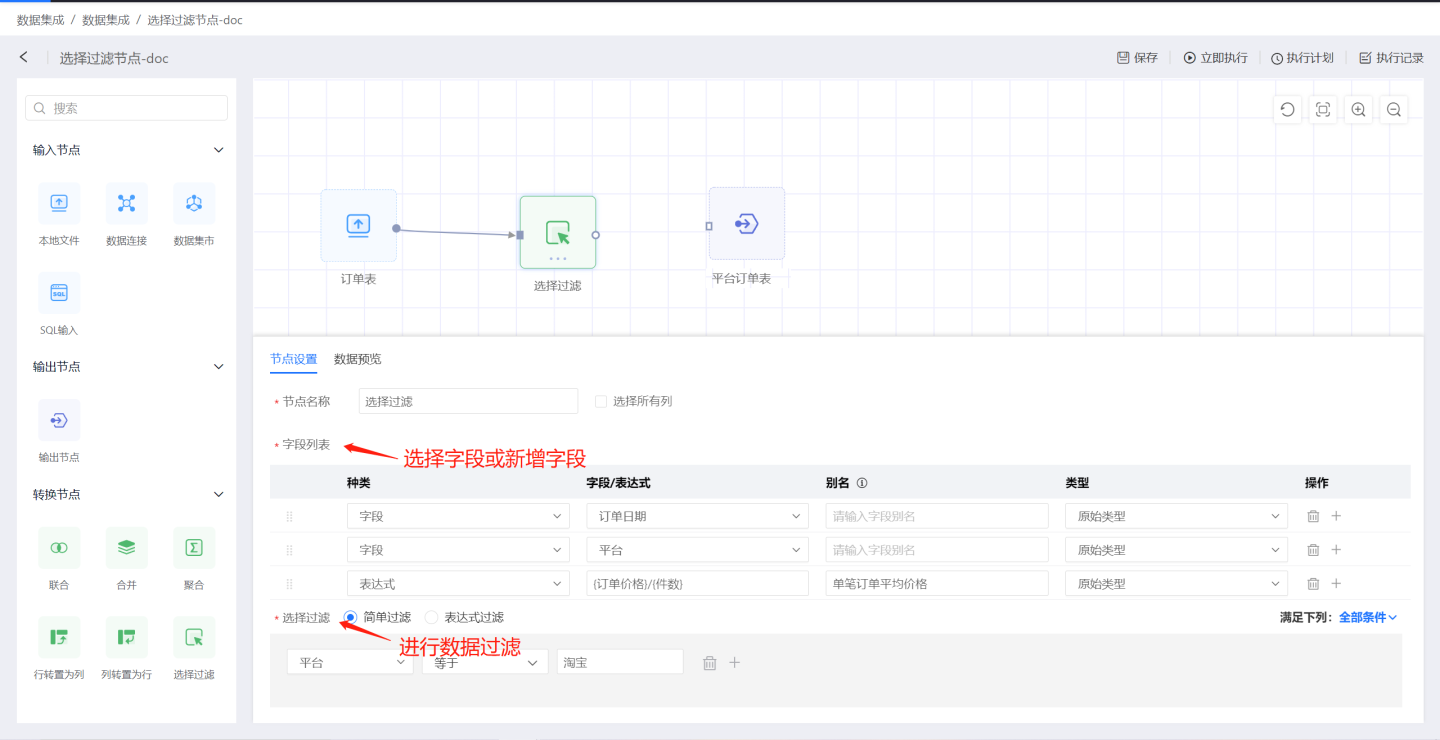
Explanation of Select Filter configuration:
Node Name: Default is
Select Filter, and users can modify it.Select All Columns: When checked, all columns in the input data are added to the output data but are not displayed in the field list.
Field List: Allows users to add column fields. Supports adding original fields and creating new fields using expressions.
- Field: Adds original fields from the input data, with options to modify aliases and field types. If
Select All Columnsis checked, please modify the alias when adding fields to avoid duplicate field names. - Expression: Creates new fields using expressions.
- Field: Adds original fields from the input data, with options to modify aliases and field types. If
Filter Method
- Simple Filter: Users set filtering conditions through options. When there are multiple filtering conditions, users can choose the condition selection method: 'All Conditions' or 'Any Condition'. 'All Conditions' means the filtered data must meet all filtering conditions. 'Any Condition' means the filtered data only needs to meet one of the conditions.
- Expression Filter: Users set filtering conditions using expressions for more flexible data filtering. The filtering expression must return a Boolean value. On the right side of the expression editing area is a function list available for use in expressions.
Typical usage scenarios for the Select Filter node:
Scenario 1: Add fields using
Select All Columnsand set filtering conditions without adding fields in the field list.
As shown in the figure, onlySelect All Columnsis checked, and no fields are added to the field list. Simple filtering is used to filter out data where the platform is Xiaohongshu.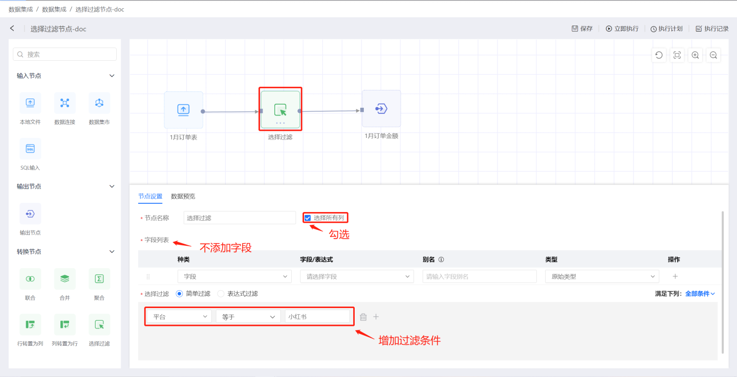
The output result is shown in the figure, containing all field information from the input data and filtering out data where the platform is Xiaohongshu.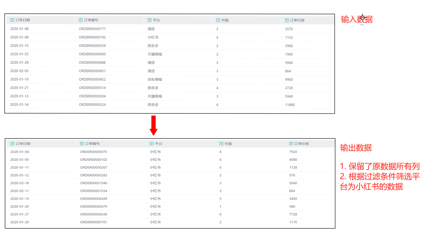
Scenario 2: Add fields in the
Field Listand filter the fields.
As shown in the figure, the original fieldsOrder DateandPlatformare selected in the field list, and a new fieldUnit Priceis created using an expression.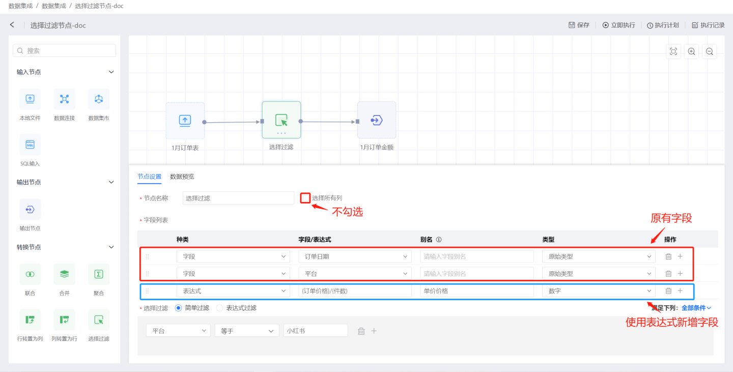
The output result is shown in the figure, containing only the three fields created in the field list and filtering out data where the platform is Xiaohongshu based on the filtering conditions.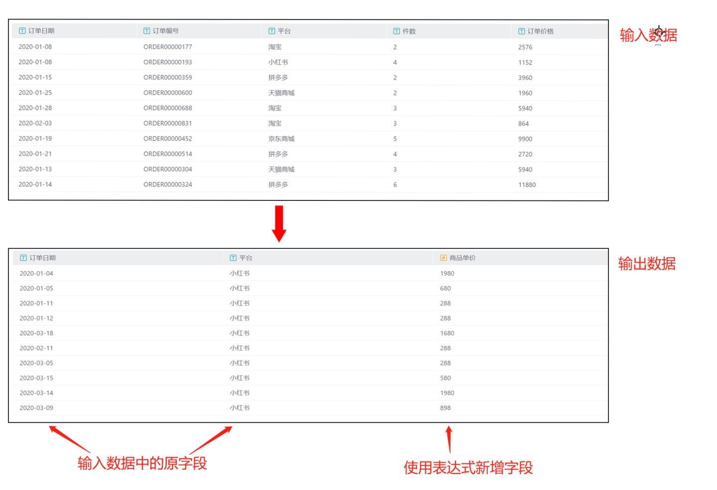
Scenario 3: Add fields using both
Select All ColumnsandField Listand set filtering conditions.
As shown in the figure,Select All Columnsis checked, and the original fieldsOrder DateandPlatformare added to the field list, with aliases and types modified. A new fieldUnit Priceis created using an expression.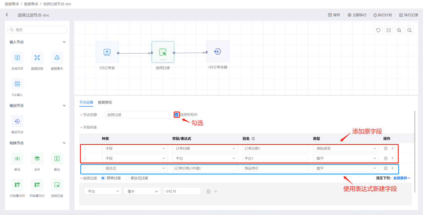
The output result is shown in the figure, containing all fields from the input data as well as the three fields created in the field list. The data is filtered based on the filtering conditions to include only data where the platform is Xiaohongshu. The fieldsOrder DateandPlatformin the field list are original fields added, which conflict with the field names inSelect All Columns, so aliases need to be modified.Platform1underwent a numeric type conversion, which failed, so null values are used for filling.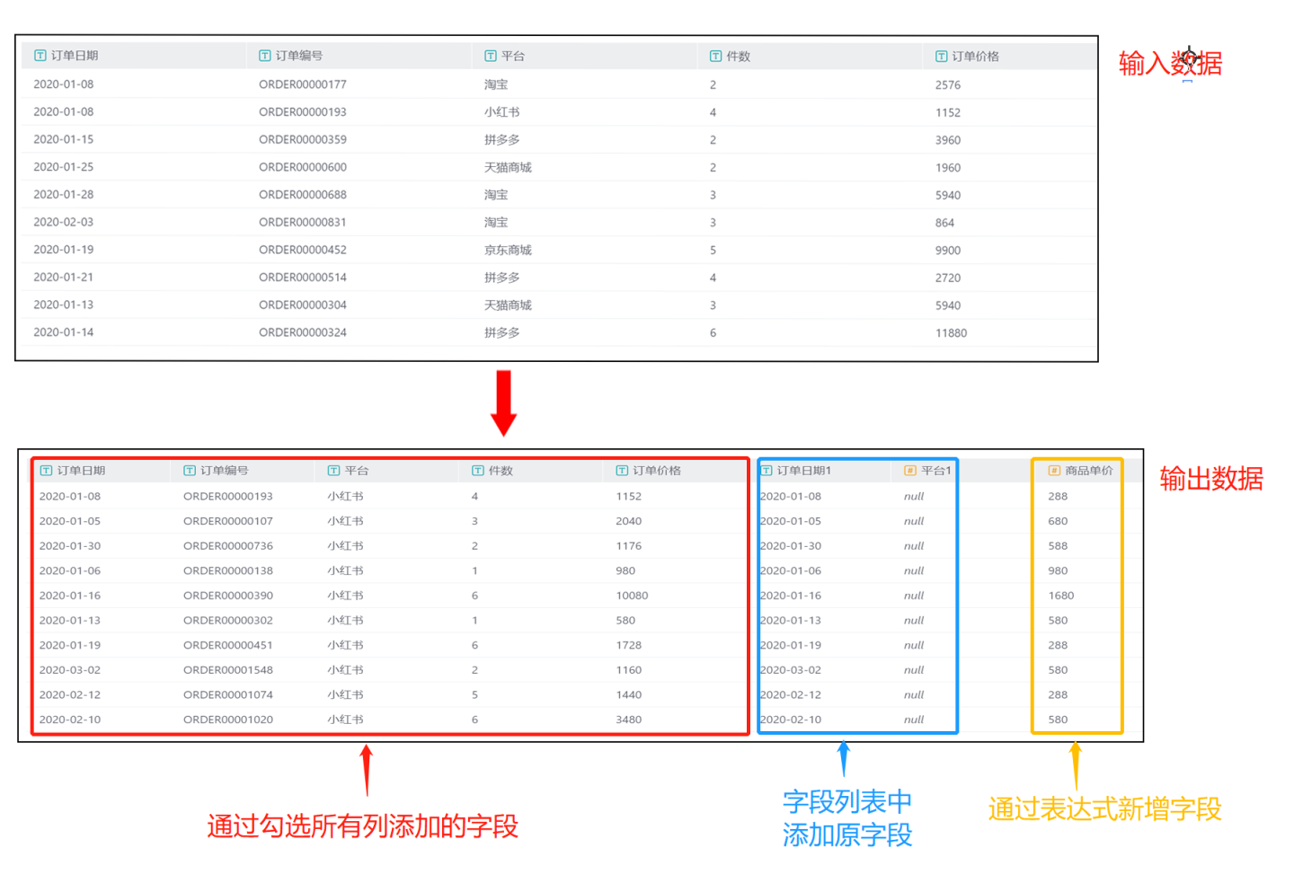
Transpose Rows to Columns
Transposing rows to columns involves converting the values of a specific row in the input data into columns for display. As shown in the figure, the values of the platform field, such as Taobao, Tmall Mall, and JD Mall, are converted into column names to view the total order cost for these three platforms. 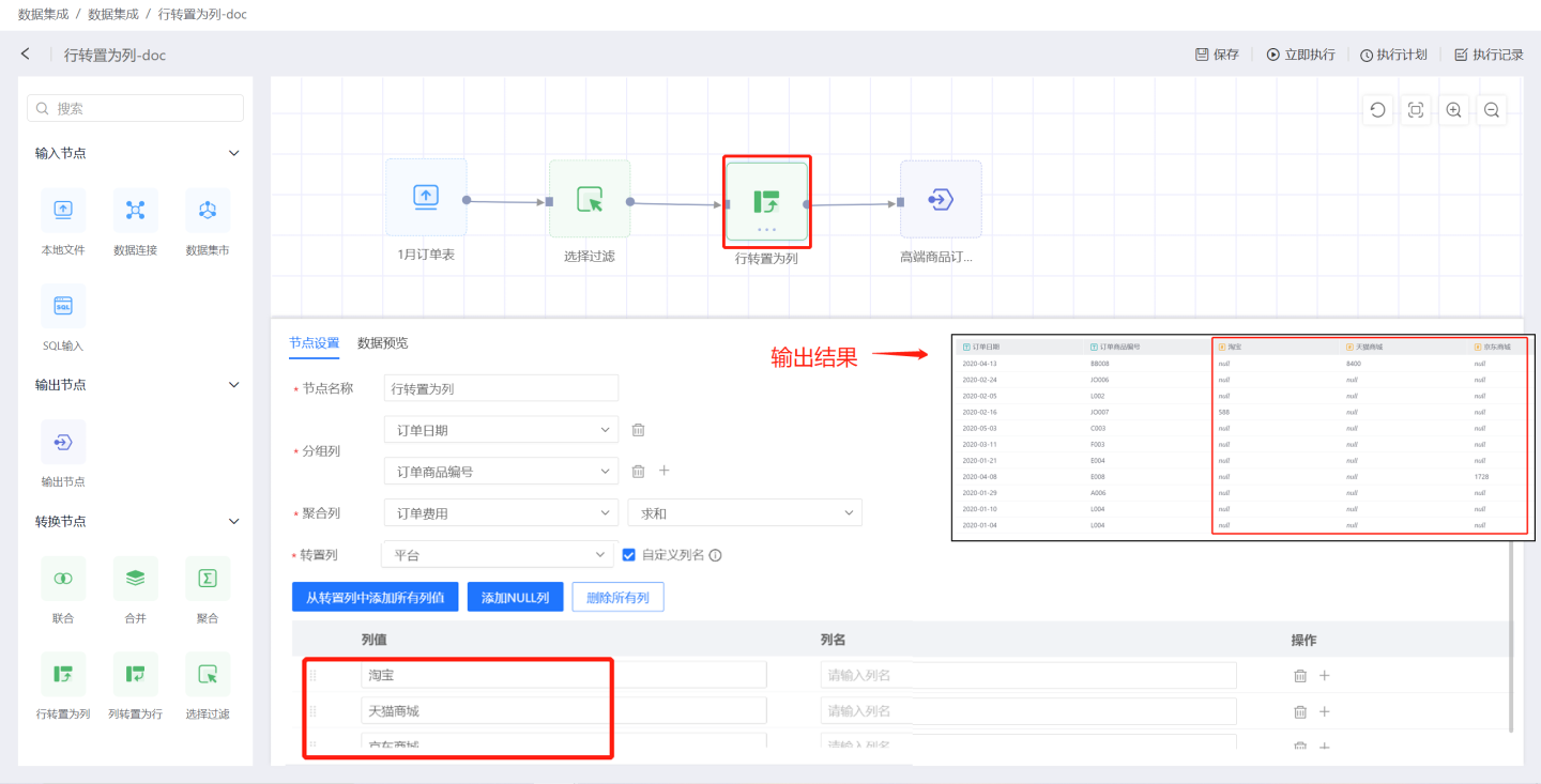
Configuration details for the "Transpose Rows to Columns" node:
- Node Name: Default is
Transpose Rows to Columns, but users can modify it. - Group Columns: Adds the original fields from the input data to the output data. You can add one or more fields.
- Aggregate Columns: The values of the aggregate column are used to populate the transposed columns. When the aggregate column is of numeric type, it supports operations such as average, sum, maximum, minimum, count, and deduplication. For non-numeric types, it supports maximum, minimum, count, and deduplication.
- Transpose Column: Specifies the field to be transposed into columns. By default, the values of this field will be presented as columns. Users can customize column names. You can manually add column value fields or use shortcut buttons for operations.
- Add All Column Values from Transpose Column
Displays all column values of the transpose column field. You can use the delete button to select the column values you need for conversion and modify aliases. - Add NULL Column
Adds a column with NULL values. - Delete All Columns
Deletes all column information displayed in the list.
- Add All Column Values from Transpose Column
Typical use cases for the "Transpose Rows to Columns" node in data integration:
Scenario 1: Using the default method, all values in the transpose column are displayed as columns without customizing column names.
In the example, the node configuration adds group columnsOrder DateandOrder Product ID. All column values in the transpose columnPlatformare converted into column names, and the sum ofOrder Costin the aggregate column is used to populate the transposed column values.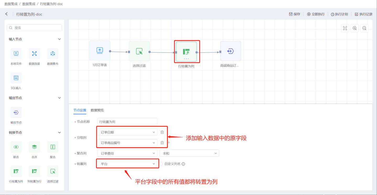
The output includes the original data columnsOrder DateandOrder Product ID, and all values in thePlatformcolumn are converted into columns (red box). These column values are populated using the sum ofOrder Cost(blue box).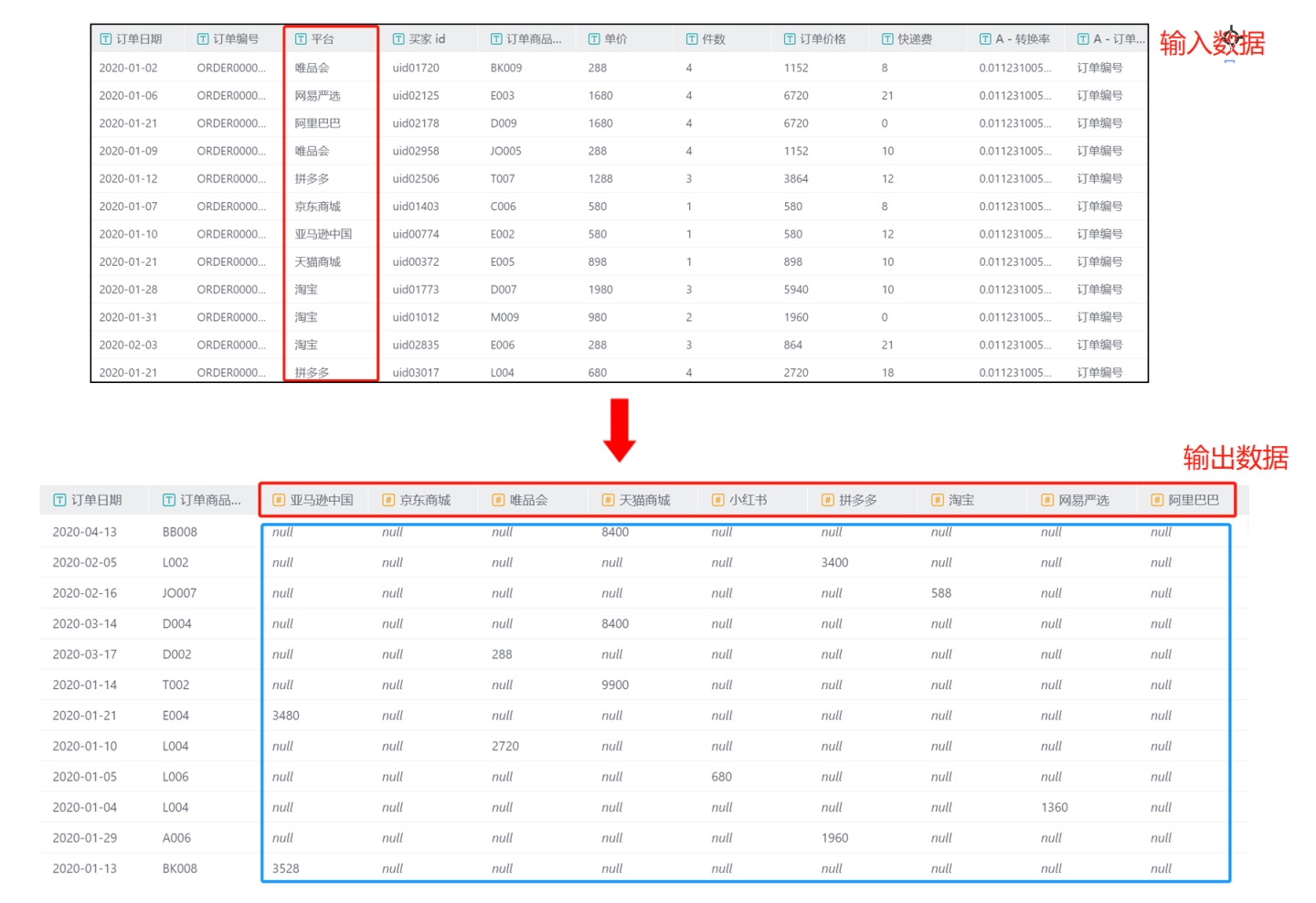
Scenario 2: Manually adding column values for the transpose column, including values not in the original transpose column.
In the example, column valuesTaobao,Tmall Mall,JD Mall,NULL, andWeidianare manually added to the platform column.NULLandWeidianare not values in the original transpose column.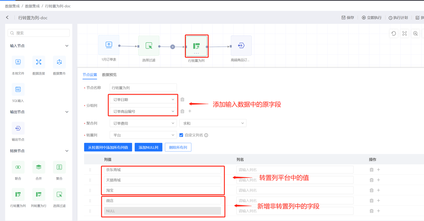
The output includes the original data columnsOrder DateandOrder Product ID, as well as the column valuesTaobao,Tmall Mall, andJD Mallfrom thePlatformcolumn, populated using the sum ofOrder Cost.NULLandWeidianare values not in the transpose column, and since there is noOrder Costinformation for these fields in the original data, they are filled with null values.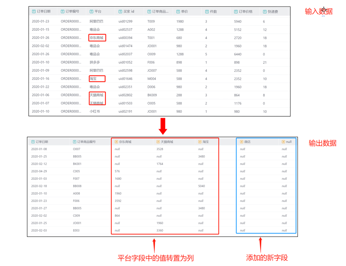
Transpose Columns to Rows
Transposing columns to rows involves summarizing certain columns with common characteristics in the input data and converting them into rows for display. As shown in the figure, Robot, Manipulator, Auxiliary Machine, Water and Gas are all part of components, which are organized into the Components column for display. 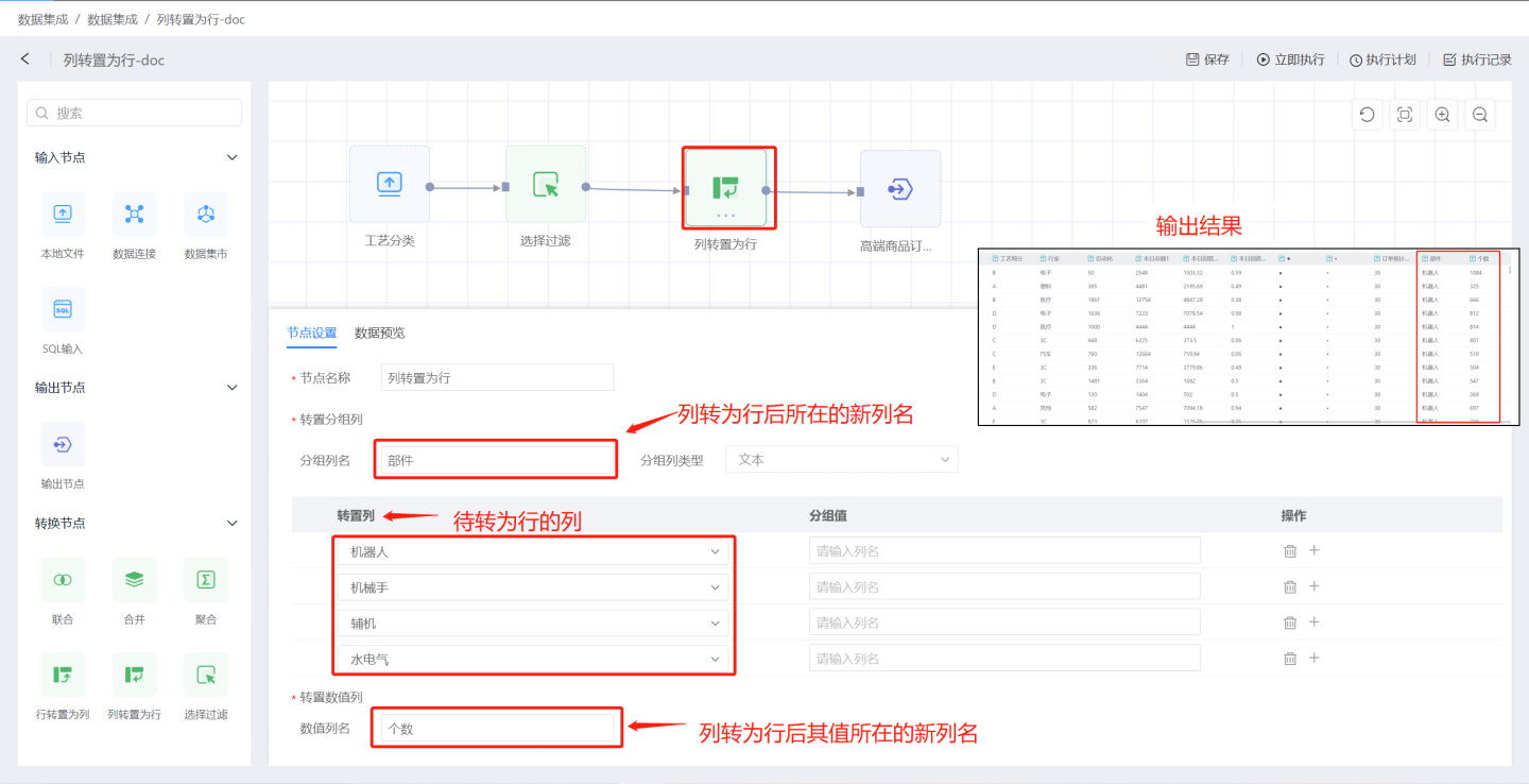
Configuration details for the Transpose Columns to Rows node:
- Node Name: Default is
Transpose Columns to Rows, and users can modify it. - Transpose Group Columns:
- Group Column Name: The field name after transposing columns to rows. Group column types include text, number, and date. Transpose columns are the columns to be converted into rows, and group values can be modified. Multiple transpose columns are supported.
- Transpose Value Column: The name of the new column where the values of the transposed columns will be stored.
Typical use cases for the dataset Transpose Columns to Rows node:
- Scenario 1: Convert columns with common characteristics into groups for display and modify the group values after conversion. In the example, columns such as
Robot,Manipulator,Auxiliary Machine,Water and Gas, andAutomationare converted into rows stored in the new columnComponents, and the values of these columns are stored in the new columnCount. Among them, the names of the columnsWater and GasandAutomationare modified toWater and Gas EquipmentandAutomation Componentsafter conversion.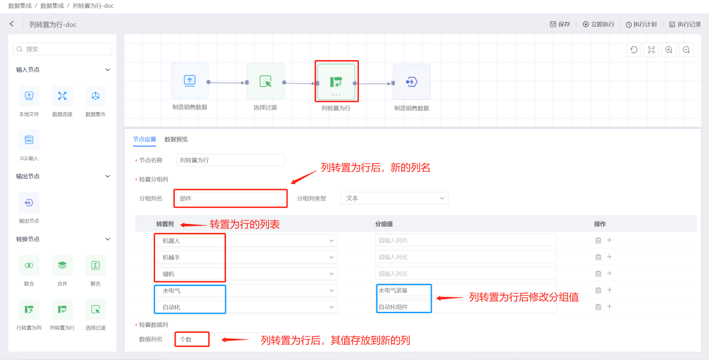 The output result is shown in the figure. After transposing, columns such as
 Robot,Manipulator,Auxiliary Machine,Water and Gas, andAutomationare stored in theComponentscolumn, and their values are stored in theCountcolumn.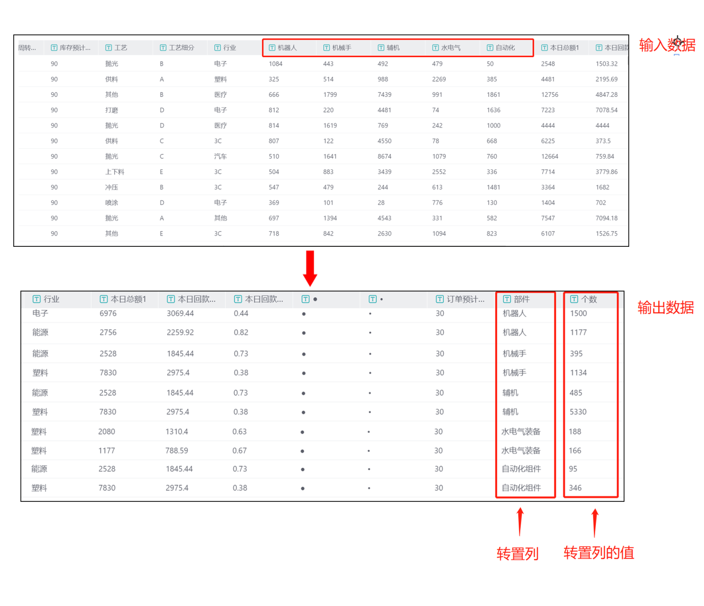
Project Execution
After all data nodes in the data integration project are created, the project can be executed. Each project supports two triggering methods: immediate execution and scheduled execution.
Execute Immediately
Clicking Execute Immediately will add the project to the execution queue for processing, and the button will change to Stop Execution.
Tip
Depending on the task queue situation, after clicking Execute Immediately, the project may be in either Queued or Executing status.
Queued: For projects in the Queued status, clicking Stop Execution will cancel the current execution.
Executing: For projects in the Executing status, the action button is disabled, and execution cannot be canceled. You must wait for the current execution to complete.
Execution Plan
Click on the execution plan in the upper right corner to enter the execution plan settings page, where you can configure the basic information, scheduling information, and alert information for the plan.
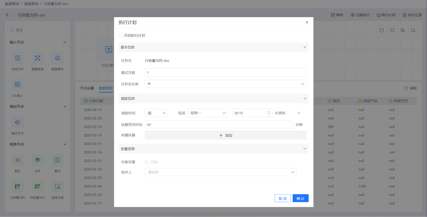
- Basic Information: Configure the retry count and task priority during execution. Task priority is divided into three levels: high, medium, and low. Tasks with higher priority are processed first.
- Scheduling Information:
- Set the task scheduling time, and multiple scheduling times can be configured. Supports scheduling plans by hour, day, week, or month.
- Hour: You can set updates at specific minutes of each hour.
- Day: You can set updates at specific times of each day.
- Week: You can set updates at specific times on specific days of the week, with multiple selections allowed.
- Month: You can set updates at specific times on specific days of the month, with multiple selections allowed.
- Custom: You can manually configure update times.
- Configure task dependencies, allowing multiple prerequisite tasks to be set.
- Set dependency wait time.
- Set the task scheduling time, and multiple scheduling times can be configured. Supports scheduling plans by hour, day, week, or month.
- Alert Information: Enable failure alerts. When a task fails to execute, an email notification will be sent to the recipient.
Execution Records
Click on Execution Records in the upper right corner of the project to view all execution records of the project.
Daily Project Operations
Data integration projects support operations such as creating new projects, editing, executing immediately, creating copies, deleting, filtering, and searching. Immediate execution refers to the Immediate Execution feature of the project, which will not be elaborated on here.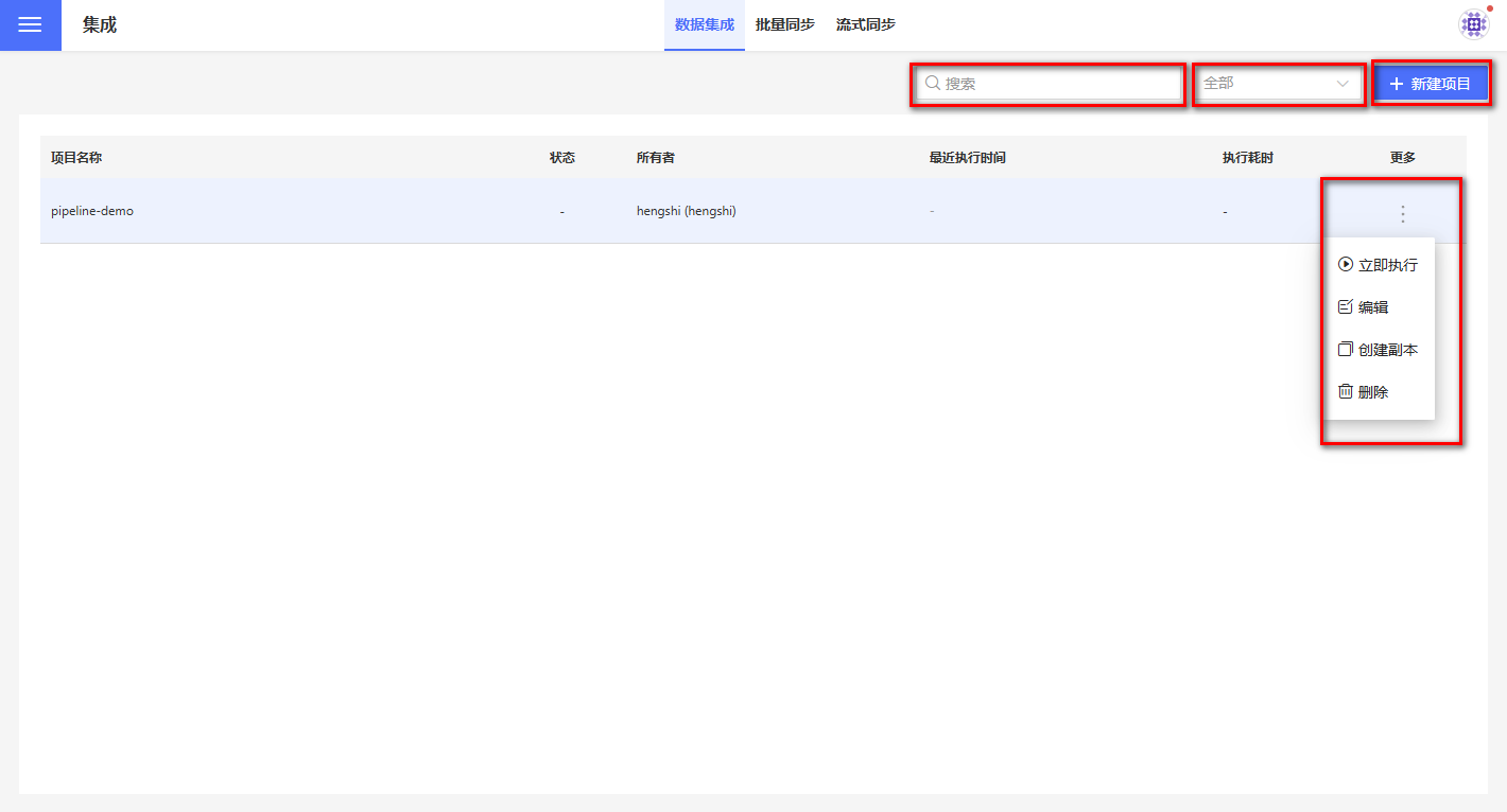
Create a New Project
Click on Create Project in the upper right corner to open the project creation dialog box. Enter the project name in the popup window and select the default output path for the project from the available data connections in the Default Output Path dropdown menu.
Note:
The list of connection types that support data connections as default output paths is the same as the list supported in Output Node.
For connections that can be used as output paths for data integration, the owner must check the Allow Write Operations option when creating the connection; otherwise, the output table cannot be stored.
Edit Project
Click the edit button in the three-dot menu under the More column corresponding to the project. In the pop-up edit box, you can modify the project's name and the default output path.
Delete Project
Click the Delete button in the three-dot menu under the More column for the corresponding project. A confirmation box will pop up; click confirm to delete the project.
Filter Items
Project filtering supports classification based on the execution status of the project. The dropdown menu for execution status includes:
- All
- Success
- Failure
- Queued
- Canceled
- Running
It supports searching for projects containing keywords under specified filtering conditions. For example, searching for Failure projects containing the keyword "Dataset" among all projects.
FAQ
- Nodes in the canvas area with a red lightning icon indicate execution errors, while a red exclamation mark indicates configuration errors. Please check the node configuration and make the necessary modifications.
- The data processing flow for output nodes is:
Pre-load SQL -> Schema Validation -> Table Operations -> Update Method -> Post-load SQL. - If a node fails to execute in a project, the entire project stops execution.
- When the input node data extraction is empty, subsequent steps will not be executed.